Confluent hypergeometric function
In mathematics, a confluent hypergeometric function is a solution of a confluent hypergeometric equation, which is a degenerate form of a hypergeometric differential equation where two of the three regular singularities merge into an irregular singularity. (The term "confluent" refers to the merging of singular points of families of differential equations; "confluere" is Latin for "to flow together".) There are several common standard forms of confluent hypergeometric functions:
- Kummer's (confluent hypergeometric) function M(a,b,z), introduced by Kummer (1837), is a solution to Kummer's differential equation. There is a different but unrelated Kummer's function bearing the same name.
- Tricomi's (confluent hypergeometric) function U(a;b;z) introduced by Francesco Tricomi (1947), sometimes denoted by Ψ(a;b;.z), is another solution to Kummer's equation.
- Whittaker functions (for Edmund Taylor Whittaker) are solutions to Whittaker's equation.
- Coulomb wave functions are solutions to Coulomb wave equation.
The Kummer functions, Whittaker functions, and Coulomb wave functions are essentially the same, and differ from each other only by elementary functions and change of variables.
Contents |
Kummer's equation
Kummer's equation is
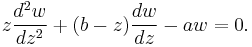 ,
,
with a regular singular point at 0 and an irregular singular point at ∞. It has two linearly independent solutions M(a,b,z) and U(a,b,z).
Kummer's function (of the first kind) M is a generalized hypergeometric series introduced in (Kummer 1837), given by
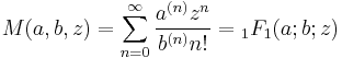
where

is the rising factorial. Another common notation for this solution is Φ(a,b,z). This defines an entire function of a.b, and z, except for poles at b = 0, −1, − 2, ...
Just as the confluent differential equation is a limit of the hypergeometric differential equation as the singular point at 1 is moved towards the singular point at ∞, the confluent hypergeometric function can be given as a limit of the hypergeometric function
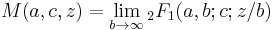
and many of the properties of the confluent hypergeometric function are limiting cases of properties of the hypergeometric function.
Another solution of Kummer's equation is the Tricomi confluent hypergeometric function U(a;b;z) introduced by Francesco Tricomi (1947), and sometimes denoted by Ψ(a;b;.z). The function U is defined in terms of Kummer's function M by

This is undefined for integer b, but can be extended to integer b by continuity.
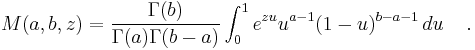
Integral representations
If Re b > Re a > 0, M(a,b,z) can be represented as an integral
For a with positive real part U can be obtained by the Laplace integral

The integral defines a solution in the right half-plane re z > 0.
They can also be represented as Barnes integrals
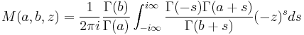
where the contour passes to one side of the poles of Γ(−s) and to the other side of the poles of Γ(a+s).
Asymptotic behavior
The asymptotic behavior of U(a,b,z) as z → ∞ can be deduced from the integral representations. If z = x is real, then making a change of variables in the integral followed by expanding the binomial series and integrating it formally term by term gives rise to an asymptotic series expansion, valid as x → ∞:[1]
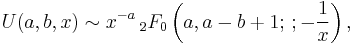
where 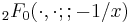 is a generalized hypergeometric series, which converges nowhere but exists as a formal power series in 1/x.
Relations
There are many relations between Kummer functions for various arguments and their derivatives. This section gives a few typical examples.
Contiguous relations
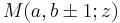
Given  , the four functions
 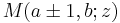 ,
,  are called contiguous to . The function can be written as a linear combination of any two of its contiguous functions, with rational coefficients in terms of
  ,
, and
and  . This gives (4
2)=6 relations, given by identifying any two lines on the right hand side of
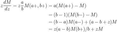
In the notation above,  and so on.
Repeatedly applying these relations gives a linear relation between any three functions of the form 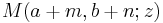 (and their higher derivatives), where
  ,
,  are integers.
There are similar relations for U.
Kummer's transformation
Kummer's functions are also related by Kummer's transformations:

 .
.
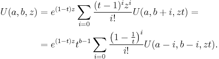
Multiplication theorem
The following multiplication theorems hold true:
Connection with Laguerre polynomials and similar representations
In terms of Laguerre polynomials, Kummer's functions have several expansions, for example
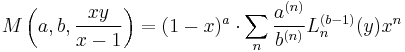 (Erdelyi 1953, 6.12)
Special cases
Functions that can be expressed as special cases of the confluent hypergeometric function include:
- Bateman's function
- Bessel functions and many related functions such as Airy functions, Kelvin functions, Hankel functions.
For example, the special case  the function reduces to a Bessel function:
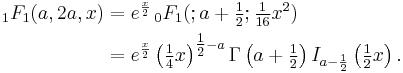
This identity is sometimes also referred to as Kummer's second transformation. Similarly
where  is related to Bessel polynomial for integer .
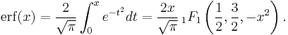
- The error function can be expressed as
- Coulomb wave function
- Cunningham functions
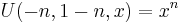
- Elementary functions such as sin, cos, exp. For example,
- Exponential integral and related functions such as the sine integral, logarithmic integral
- Hermite polynomials
- Incomplete gamma function
- Laguerre polynomials
- Parabolic cylinder function (or Weber function)
- Poisson–Charlier function
- Toronto functions
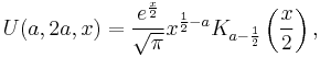
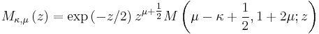
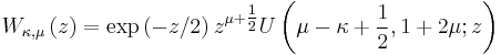
- Whittaker functions Mκ,μ(z), Wκ,μ(z) are solutions of Whittaker's equation that can be expressed in terms of Kummer functions M and U by
- The general p-th raw moment (p not necessarily an integer) can be expressed as
-
![\operatorname{E} \left[\left|N\left(\mu, \sigma^2 \right)\right|^p \right]= \left(2 \sigma^2\right)^\frac p 2 \frac {\Gamma\left(\frac{1%2Bp}2\right)}{\sqrt \pi}\, _1F_1\left(-\frac p 2, \frac 1 2, -\frac{\mu^2}{2 \sigma^2}\right),](/2012-wikipedia_en_all_nopic_01_2012/I/42729d900168e9c3309da46311255891.png)
![\operatorname{E} \left[N\left(\mu, \sigma^2 \right)^p \right]=(-2 \sigma^2)^\frac p 2 \cdot U\left(-\frac p 2, \frac 1 2, -\frac{\mu^2}{2 \sigma^2} \right)](/2012-wikipedia_en_all_nopic_01_2012/I/1ede10496c3be877357b3b5802e7cbcf.png) (the function's second branch cut can be chosen by multiplying with
(the function's second branch cut can be chosen by multiplying with  ).
).
Application to continued fractions
By applying a limiting argument to Gauss's continued fraction it can be shown that
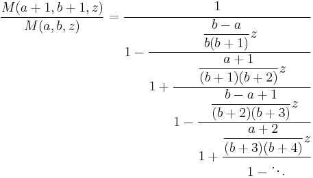
and that this continued fraction converges uniformly to a meromorphic function of z in every bounded domain that does not include a pole.
Notes
- ^ Andrews, G.E.; Askey, R.; Roy, R. (2000). Special functions. Cambridge University Press.
References
- Abramowitz, Milton; Stegun, Irene A., eds. (1965), "Chapter 13", Handbook of Mathematical Functions with Formulas, Graphs, and Mathematical Tables, New York: Dover, pp. 504, ISBN 978-0486612720, MR0167642, http://www.math.sfu.ca/~cbm/aands/page_504.htm.
- Chistova, E.A. (2001), "Confluent hypergeometric function", in Hazewinkel, Michiel, Encyclopedia of Mathematics, Springer, ISBN 978-1556080104, http://www.encyclopediaofmath.org/index.php?title=c/c024700
- Daalhuis, Adri B. Olde (2010), "Confluent hypergeometric function", in Olver, Frank W. J.; Lozier, Daniel M.; Boisvert, Ronald F. et al., NIST Handbook of Mathematical Functions, Cambridge University Press, ISBN 978-0521192255, MR2723248, http://dlmf.nist.gov/13
- Erdélyi, Arthur; Magnus, Wilhelm; Oberhettinger, Fritz & Tricomi, Francesco G. (1953). Higher transcendental functions. Vol. I. New York–Toronto–London: McGraw–Hill Book Company, Inc.. MR0058756.
- Kummer, Ernst Eduard (1837). "De integralibus quibusdam definitis et seriebus infinitis" (in Latin). Journal für die reine und angewandte Mathematik 17: 228–242. ISSN 0075-4102. http://resolver.sub.uni-goettingen.de/purl?GDZPPN002141329.
- Slater, Lucy Joan (1960). Confluent hypergeometric functions. Cambridge, UK: Cambridge University Press. MR0107026.
- Tricomi, Francesco G. (1947). "Sulle funzioni ipergeometriche confluenti" (in Italian). Annali di Matematica Pura ed Applicata. Serie Quarta 26: 141–175. ISSN 0003-4622. MR0029451.
- Tricomi, Francesco G. (1954) (in Italian). Funzioni ipergeometriche confluenti. Consiglio Nazionale Delle Ricerche Monografie Matematiche. 1. Rome: Edizioni cremonese. ISBN 9788870834499. MR0076936.
External links
- Kummer hypergeometric function on the Wolfram Functions site
- Tricomi hypergeometric function on the Wolfram Functions site